The spacecraft angular velocity estimation in the orbital stabilization mode by the results of the local vertical sensor measurements

8 / 11

Jy = 274021 ; Jz = 238845, and with the usage of a set of units (SI)
the initial values of SC state vector are equal γ ωx ψ ωy
T =
= 0,1 0,005 − 0,1 0, 002
T; ϑ ωz
T
= 0,1 0 ,003
T. As an
initial approximation of estimation values for the angular velocity vector
let’s choose the beginning of coordinates: ˆ ωx0 ˆ ωy 0
T
= ( 0, 0 0, 0 )T;
ˆ ωz 0 = 0,0.
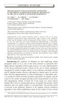
The simulation results are given in Figure 1, which presents the change
of non-correction components of angular velocity vector (˜ ωx = ωx − ˆ ω x,
˜ ωy = ωy − ˆ ωy , ˜ ωz = ωz − ˆ ωz ) in accordance with the iteration index.
The range of non-connection changes (part a and b of the figure) is
quite large and correspondingly it is difficult to estimate the convergence
accuracy of SC angular rotation velocity vector using the given dependencies,
that is why starting from the fourth tact of iteration process, the simulation
results are presented in Table 1.
Table 1
Results of simulation
Non-connection component
of angular rotation velocity
vector, 1/s
Iteration index
4 5 6 7 8 9 10
ˆ ωx – 0.0110 0.0343 – 0.0179 0.0089 0.0050 0.0050 0.0050
˜ ωx = ωx − ˆ ωx 0.0160 – 0.0293 0.0229 – 0.0039 0.0000 0.0000 0.0000
ˆ ωy 0.0020 0.0020 0.0020 0.0020 0.0020 0.0020 0.0020
˜ωy = ωy − ˆ ωy 0.0000 0.0000 0.0000 0.0000 0.0000 0.0000 0.0000
ˆ ωz 0.0030 0.0030 0.0030 0.0030 0.0030 0.0030 0.0030
˜ ωz = ωz − ˆ ωz 0.0000 0.0000 0.0000 0.0000 0.0000 0.0000 0.0000
The analysis of the data presented in Figure 1 and Table 1 shows that
during eight iterations angular velocity vector agrees with the real value of
angular velocity vector of a SC.
Conclusion. In the present article the exact pole placement method
enables the analytical solution of SC angular velocity estimation synthesis
in a mode of orbital stabilization by the results of the local vertical
sensor measurements. The results of mathematical simulation are presented,
confirming the high algorithm efficiency. In accordance with the analysis
of computational expenses of the algorithm based on the expression (16)
and the number of iterations providing the convergence of the process by
the simulation results it may be concluded that its realization is feasible in
real time.
10 ISSN 0236-3933. HERALD of the BMSTU. Series “Instrument Engineering”. 2014. No. 5